Activity 7 – Image Segmentation

In this activity, we learn how to segment images into objects containing particular characteristic, in this activity, let’s do colors.

So let’s begin with something basic, grayscale images.

Let’s look at this particular image of a very funny check.

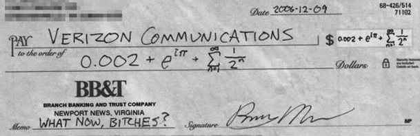
It’s so funny though.

If we look at the image, the gray background is not really useful. let’s fix this by binarizing the image. We’ll set a threshold. any pixel above this threshold level will be 0 and below is 1.  so let’s try this

Threshold = 100. We see most of the details. But some details, like the signature, are lost.

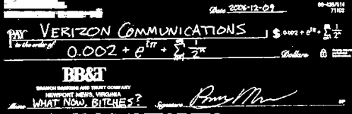
Threshold = 144. We see most of the details clearly. 

Threshold = 200. the image is too filled with white

that was easy enough. obviously, segmenting is a matter of setting the optimal threshold. but how can you find the optimal threshold at all.

well, you can just find the background pixel value. let’s look at the histogram of the image.

So the last of the background seems to be somewhere around 170. 

We take a segmented image near that

A lot more detail is visible now. The letters at the bottom-right corner are readable again

COLOR SEGMENTATION

Now let’s look at something trickier: real colored images. I thought of doing something fun. Like m&m’s.

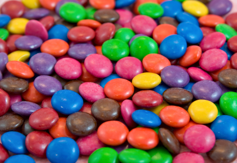
Let’s say a certain internet monster, Bernie, only eats blue m&m’s.  But a mean troll traps him and will only let him eat the blue m&m’s if Bernie can say how many there are in the picture. The problem is, Bernie has poor eyesight. Colors begin blurring around. Individually, he can distinguish blue m&m’s but they become hidden in the image. How can we help our poor friend?

This is Bernie

Well there are two ways by which we do this. The parametric, and the non-parametric segmentation method.

But here’s a problem. Graylevel segmentation works with a threshold over a single variable. Color, as humans perceive it is trichromatic. That is, color is composed of three components. It’s commonly Red Green and Blue. So how do we determine if a pixel value is the same color? since there are three channels, setting a threshold value for all three becomes hard and very difficult. Let’s see if it can be simplified.

We’ll come back to the segmentation part. Since the problem of the material is 3 channels (all of which vary from pixel to pixel due to intensity brightness). we’ll do chromacity.

Let’s say a pixel has R, G and B values. We say the intensity, I, of the pixel is I = R+G+B. We say the chromacity r = R/I as well as g = G/I. Consequently, b = B/I = 1 – r -g, so it isn’t independent anymore. We can define any color only using r and g.

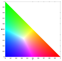
Well, you see most colors and you can represent blue without taking the chromacity of blue. Image Source: Wikipedia

So the 3-color problem is now a 2D problem.Seems easy enough. Let’s get back to Bernie’s dilemma.

Bernie can see the Blue m&m’s in the front. So he hopes to just use a quick bit of programming to find the other blue m&m’s. He takes one of the obviously blue m&m’s and studies the color.

(This photo is already zoomed in)You see that there are different shades of blue with varying values of R, G and B due to varying intensities.

So using we use this region first. We assume that this small Region Of Interest(ROI) contains, more or less, all shades of blue. We go back to something I said earlier the parametric and non-parametric methods.

Parametric

The parametric method basically means solving the probability that each pixel is the same color as the ROI. So for this we take  μ (mean value)  σ (standard deviation) in r and g of the ROI.

Then solve for the probability

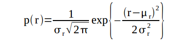
and the same for g. The probability the pixel is the same color as the ROI is then the product of the two probabilities.

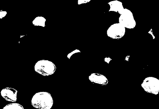
Bernie does this and comes up with

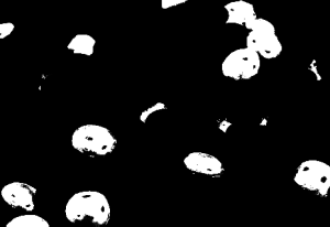
even barely visible blue m&m’s become apparent now. 

Non-parametric

Well, something easier. instead of solving probabilities(that the computer still has to round out to assign discrete RGB values to). We make a histogram of the chromacity space. therefore, with larger images, we can just look up the histogram and not have to calculate so many joint probabilities.

Bernie also does this (just to be sure) histogram

 

If you look at the normalized chromacity coordinates. It’s in the blue region.

And using this histogram Bernie got

they’re more pronounced now

So Bernie guesses right. and is able to get all the blue m&m’s he can eat.

Acknowledgements:

I would like to thank Carlo Solibet, who was nearest to me and noticed the one bug in my code that wouldn’t let me find the histogram.

I would give myself 10/10. because this activity was easy enough to do.

Activity 6 – Applications and properties of the Fourier transform

This activity, we do a lot of Fourier Transforms. We find out first how they behave so we can use that, because otherwise, it’s not really science.

A. Anamorphic Property

The great thing about the fourier transformn is that we can more or less predict what it will look like given the original dataset. to show this, let’s look at some things

Left: Original Image, Right: FFT

We see that the rectangle’s fft is wider the narrower the dimension is ( a tall rectangle’s fft is wider than that of a wide one). We also see the two bringing two dots together increase the spacing between the bands.

B. Rotation property of the fourier transform. 

Let’s start with a sinusoid along the x axis. Since this has a fixed frequency, we should see just dots in its FT

Left, original. Right, FFT

Well, as expected, the FFT are dots, as to why there are two, well it’s because the frequency could both be positive and negative. But here is where it gets interesting. What if we multiply them?

Well,. now we see repetition in the Frequency space. What if we rotate the image?

That’s interesting, the FT rotates as well.  Let’s make it more interesting. Let’s take these images,

and add them into

Since, respectively, their FTs are:

and FT is linear, we expect them to just add up

Well. Isn’t that handy? Now we know if we take the FT, we just remove the frequencies we don’t like and they should disappear after and inverse Fourier Transform.

C. Convolution Theorem Redux

We return to convolution. Apparently, aside from simulations of apertures and edge detection, we can use it in another way. Let’s look at the effect of changing distances between two dots.

We see that the resulting bandsa just get closer and closer. Let’s replace the dots with circles

We see that increasing the radius gets a smaller radius in the fft, but it also looks like there’s a sinusoid imposed. Let’s check for another shape

As we increase the width of the squares, the FFT looks more and more like the FFT of a single squatre aperture. but It also still has the sinusoidal FFT of the single dot. Let’s try a gaussian curveThe FFT still looks like that of the Gaussian curve but now there is still that sinusoid.Maybe we can use that.

Let’s use a random pattern

Just a bunch of random 1s in a 200X200 grid. I’ll use a small pattern

And convolve this with the random pattern.

Now, I get it. This is the property of the Dirac delta. In this example, the 1s are random dirac deltas. For more information, we can follow here. This could be really useful for automation in editing softwares. We can just replace regularly occuring objects(say pimples in a face).

D. Fingerprint enhancement

Let’s use what we learned in part C in something real

My fingerprint is kinda hard to determine. there are a lot of blotches from the ink and the ridges are kinda blurry. But I think since this is a repeating pattern, these blotches and ridges must be easier to separate in Frequency space.

Aha. Since the blotches are thick dots, the must contribute to the bright spot in the middle. Which means we can filter it out using

Which hopefully results in something useful for solving cases

Left: Original,. Right Filtered.

Well, it isn’t really clean. But the ridges are deifinitely clearer. Not bad since I used MS paint and didn’t binarize the image.

E. Lunar Landing Images with lines

The following image is one of the greatest testaments to mankind’s ingenuity.

We got to look closely at something that takes light a minute to get to. If only there weren’t any lines. So using the same method as the fingerprint.

We take the FFT, use a mask, multiply the two and take the inverse

Left: FFT, Right: Mask Used

And we get

Left: Original Image, Right: Filtered Image

F. Canvas Weave Removal

Is this painting a good one? I would’t know, at least not with the canvas thread being so obvious.  maybe our new tool can help with this.

the FFT looks like

so i used this mask

that i used in MS paint. The result is kinda weird.

Activity 5 – Fast Fourier Transforms in Images

In this activity, we started with the Fast Fourier Transform. The Fourier Transform is a mathematical method of transferring data into a form that is a function of frequency. In images, which are functions in space, we Fourier transform to see the image in inverse space (also called spatial frequency). I would like to discuss how the fourier transform works, but this guy (hyperlink here) says it way better than me. All we really need to know is that we can easily imagine space because we live in normal space but there are times where it’s easier to evaluate and manipulate data if it was in the frequency space.

We’ll begin with something easy

A. The Discrete Fourier Transform

The Fourier Transform has the form of an integral over all space. And normally, Fourier transforms are done analytically on functions. But since we can’t teach computers to do that real fast, it had us stomped. Until some guys named Cooley and Tukey found a way to get the fourier transform of a finite dataset, it’s called Discrete Fourier Transform(sometimes Fast Fourier Transform). A lot of signal processing software today have some form of FFT  routines. 

Interestingly, FFTs in synthetic images can act as a lens transformation.

Let’s see what a fourier transform does to some images:

 

 Left: Original Image. Right: FFT image

So we see what I was talking about. This reminds me of lower Physics courses, light through a slit but with also through a lens. Especial;ly the double slit. It looks exactly like what you’d expect with a Yooung’s Double Slit setup.

B. Convolution

Obviously, not all operations in Frequency space is the same in Time space. In the case of the Fourier Transform, if  h= f+g in time is the same as H =F+ G (because FT is linear) but if h = fg in time, H is NOT equal to FG. In the fourier space, multiplying two functions is the equivalent of CONVOLVING (denoted by *) their inverse transforms. 

In other words, if h = f*g then H=FG.

Let’s try this on an object:

because you are one

let’s convolve it with an object, let’s call it an aperture, say a circle

because we already had one

We take their Fourier Transforms (FTs) and multiply them. Then we take the inverse Fourier Transform of the result, which is

which is basically what happens if you try to look at an image through an aperture in real life. This system is basically a simulation of a pinhole camera. It even got the the loss of intensity right. So basically, convoluting two images might be like viewing one through another.

C. Correlation

There’s another thing we can do while in Frequency space and that is Correlating two  images. Doing it involves multiplying the FTs of the images, taking the conjugate of the second, multiplying the result and taking the inverse transform again.

The result of which is

Left: Image 1, Center: Image 2 and Right: their correlation

See all the bright dots in the correlated image? Well, that’s all the As aren’t they? So correlation shows all the locations of the same patterns in the images? wow.

D. Edge Detection

We already touched on edge detection in Activity 3. This time, we’re not going skip over the edge detection part. In fact, this is all we’re going to do. In the Convolution part of this activity we “saw” the VIP image through an aperture. But what if instead, we saw it though a pattern?  say  like

A vertical stripe pattern.

This pattern should reveal sectyions in the image that follows this pattern of a vertical stripe. Well, it results in

Again flipped, but obviously conforming to the pattern.

Well we see that the image is flipped, but the edges are obvious now. That’s useful. Let’s try it on other patterns

diagonal

horizontal

spot

Left: Diagonal            Center: Horizontal           Right: Spot

 So edge must be really good depending on the pattern we use.

I would like to thank everyone who helped me. Carlo Solibet, Roland Romero for help in scilab coding. And Martin Bartolome for his blog. This was a rusj job 7/10.

Activity 4 – Length and Area Estimation in Images

In this activity, a new method of image processing was taught to us. This was using green’s theorem in area estimation.

From our Mathematical Methods courses, we know that green’s theorem is a relation between the line integral of a contour and the area bounded by the contour. this is helpful in figuring out the area of objects with weird shapes.

We begin the activity with a simple image.

Test Image, simple rectangle 430×225 px in size. The image area is 500×500 px.

We use the edge function of Scilab’s SIVP toolbox. This function automatically detects the edge of the shape(though it only takes in grayscales). Interestingly, it uses many kinds of edge detection methods and thus still requires human control(at least in choosing).

This is the edge detected by ‘sobel’ setting of the edge function

this is the ‘canny’ detected by the edge function

The left one is detected by the sobel method and the right one was detected by the canny method.

So, using the edge points(from the obciously better ‘canny’ method), we can find the contour integral of the image using the discrete form of green’s theorem

and we get the area of the rectangle.

while making the image in Paint, I set its dimensions to be 430×225 px and made sure it was centered at (250,250) that gives us an area A = 96,750 pixel. By taking the difference of the maximum and minimum value of x in list of edge points, we get a dimension of(428×225) and an area of 96300(0.5% percent away). But that would require every area we want to measure to be a rectangle. Using the green’s theorem method,  we get an area of 96,954 pixel. which is about 0.2% away from the the real value, half the error of the max – min method. Interestingly, I found that knowing the centroid improves the method’s accuracy.  In my code, the further I was from the actual centroid of the shape, the worse my measurements were.

We extended this new method to some real world applications:

I wanted to find out how big the CS Amphitheater was. So I took a screenshot of the google maps image of the amphitheater.

google maps screenshot of CS Amphitheater. Bottom corner: Map to scale.

There are two things to take here. Using Paint, I measured the number of pixels the scale bar(which corresponded to a  20 meter distance in real life). I cropped the image. Darkened the area I wanted to measure and saved it as a monochrome image.

with the centroid (calculated using midpoints of the maximum distance of the axes) at (279,290),  the area calculated using Green’s theorem = 4448.75 sq. m. Which is 0.7% away from the expected 4417 sq.m  found using the bar scale.

I’m more or less confident with the green’s method algorithm so I used it to find the area of NIP.

I don’t know if I’m right but the area calculated was 5529 sq.m.

Finally, we used an image analysis software called imageJ that has a pixel scale. As a sample I used a 50 peso bill. Using ImageJ,  I used the length of the bill as the known length and found that the width was 66.75mm(it was actually 66mm).

Additionally, I tried looking at the Republic Seal

The measurement dialog box tells me that line in yellow tells is 10.155 mm.

I think I deserve 12/10 for this activity because I did all the procedures correctly and investigated the effects of centroid placement and experimented with shapes.

Many thanks to the heroes who wrote the scilab documentation.

I had to get creative.

Activity 3 – Scilab Basics

This activity was to build up our basics in SciLab. Scilab is easier to use than most programming platforms. I found it difficult to use scilab. Possibly because the documentation of Scilab is less definite than I’m used to with python.

The goals of this activity was to learn enough about scilab to create synthetic images.

In the activity sheet, this example of synthetic image is a circle:

Scilab script for circle image. A mask r is used so that conditions upon r can be interpreted into A.

On the left is a higher res image(500×500 pixels). This was made by changing nx and ny along the image.

There was a set of challenges:

Centered Square Aperture

in order to do a centered square aperture. I changed the condition inside the find function. I set it so that every pixel that was a certain vertical distance away from the center was set to black.

Major changes from example(condition for black changed to individual axes). I found out about ‘&’.

Annulus

The annulus was simple to do. A smaller circle did the trick.

Sinusoid

The sinusoid was a bit trickier. At first I thought that the image was supposed to look like a sin wave on the xy plane. But after consulting with classmates like Angelo Rillera, I found out that the image was supposed to look like a corrugated roof.  I did it by this:

I defined an axis and set a grid the size of that axis. Then I just took the sin value over the whole grid.

Grating

At first I thought that we needed to make multiple rectangles and define each line. But I figured that you can make a square wave by making a pass filter. So I used the sine function image and included 2 conditions: anything negative is 0 and anything positive is 1.

Cross

The cross was easy. It was two rectangles.

Gaussian Aperture

The gaussian aperture was complicated. It the mask r was needed for the circular ring but the gaussian transparency had to be done on A(took me multiple trial-and-errors to find that out).

 

Activity 2 – Digital Scanning

This week, we started with Digital Scanning. We were tasked with taking an old handdrawn figure from old journals or books and use ratio and proportion to find the scale of the drawing and extrapolate data from the graph.

I took from Dr. Roland Sarmago’s PhD thesis titled: Comparative Study of the Substitution effects of rare earth ions on the electronic states and superconducting properties of Bi-2212.  The only hand-drawn image in the whole thesis was

This graph was hand written and was described in the text. It’s a piece-wise function because it’s a set of instructions to the temp-controller. Time is in hours and Temperature is in Degrees Celsius

In order to recreate this graph, every segment shown between the square dots was taken in Pixel locations.  Using Excel’s regression tools, I took the regression equation to predict further points. This is what the graph looks like

Colored lines are the regressed sample lines. All the straight lines have an R-value = 0.999 while the offset has an R-value of 0.94 with a Power function. 

The straight lines more or less are linear and react the same. The melt step(orange line) is one hour long. The growth step is 1020°C – one hour rampdown – 1007°C – one hour ramp down – 995°C. The off step, is expected to obey a power law because of Newton’s law of cooling.

Activity 1 – Basic Ratio and Proportion

For the first meeting, we did a simple activity indicating the use of ratio and proportion. We inserted ourselves into our favorite movie posters.

Can you guess which one is real?

This was done using paint. It was hard to find the specific photo that would match the facial orientation especially since none of these actors look into the lens (which is the usual etiquette for photos).